Why ZK in ZK doesn’t matter that much
ZK has by now become a snappy buzzword that sells well. Yet many of those who use it may have a very vague idea of what it is, even if they know that the acronym stands for Zero Knowledge. It is very much a paradox: while the technologies that are now assembled under the ZK umbrella do indeed emerge from an area of research dubbed “zero-knowledge proofs”, the zero-knowledge part is actually the less relevant one for many existing applications. More often than not, systems that are said to use ZK don’t have the zero-knowledge features but have something else that is now also part of the ZK “brand”.
While the original goals of ZK proofs are summed up under “Tell me your claim is true without telling me that your claim is true”, its current applications are better explained in a context of delegated computation.
In real-world applications, this shows up very concretely. Think about perpetual DEXes: complex state transitions like liquidations, trade matching, and margin checks need to be computed correctly across a large and constantly changing state.
An alternative to re-executing all of this directly on-chain is to run the computation in dedicated execution environments like Parasol, and only bring the result back on-chain. But the question is: how can we be sure that the result is correct?
This is where zero-knowledge comes into play. The original intention of zero-knowledge proofs was to wrap a statement into a sort of mathematical puzzle in such a way that one is only able to provide an answer for the puzzle if they know the original statement. Somehow, this eventually led to constructions where the puzzle is much shorter than the original statement. Thus succinct ZK proofs came into being. And that’s exactly what one needs for verifying a delegated computation. If you wrap the computation process as a succinct puzzle and provide both the results of your long computation and the answer to the puzzle, the delegating party is able to verify that the necessary computation was indeed performed. Thus, we achieve a trustless technology-based delegation scheme.
What comes after is an attempt to explain ZK proofs, or rather their succinct version, which may or (quite often) may not have the property of actually hiding information as originally intended by zero-knowledge.
A short outline of our plan is the following: we show a way to encode any computer program into a special mathematical construction that involves polynomials (and a bunch of other things). With this encoding we construct a mathematical puzzle that can only be solved by the prover if they have honestly run the program, or they are unbelievably lucky. Yet checking the answer to the puzzle is rather simple. Thus, the output of the program, together with a solution to the puzzle, forms a proof that the output was generated correctly.
The moment you need all that math from school algebra
The construction of the mathematical puzzle, conventionally named a (ZK) proof relies upon some tools from algebra. So far in this article you probably could rely upon general technical knowledge but now we’ll have to brush up on your school algebra and maybe even go beyond. The proof constructions we plan to describe will most of the time be over-simplified and a little unrealistic, but even so they’ll need a good deal of math. Yet, if “Understanding ZK proofs” is your goal, you might consider making the effort.
The key concept for constructing proofs is a polynomial: an expression with additions, multiplications (and, hence, powers), constant numbers and a variable, for instance, x. Something like this:
$$5x^3 - 2x^2 + x - 4 .$$
The value of the variable’s highest power is the polynomial degree. Hence, the polynomial above has degree 3, because it has $x^3$ in it. A value x that nullifies the polynomial is called its root. The polynomial above has $x = 1$ as a root, since:
$$5\cdot 1^3 - 2\cdot 1^2 + 1 - 4 = 5 - 2 + 1 - 4 = 0$$
A key property of polynomials that we’ll need further on relates the number of a polynomial’s roots to its degree: the number of distinct roots never exceeds the degree. The catch with this property is that it holds while we work with real numbers. But once we get into the computer world, we are doomed to have problems. This is because we imagine the set of numbers to be infinite, while there is hardly anything infinite in reality, and one thing that is bound to be finite is computer memory, especially with current prices. So, we have to limit the size of numbers we work with, which implies that there exists a “largest number”. For a 64-bit architecture that would be
$$18446744073709551615 = 2^{64}-1$$
and if you ask a computer for the result of 18446744073709551615 + 1, you get a 0. That’s what is often called an overflow. We wouldn’t care much about it, but the sad truth is that it breaks the property we intended to use. If you start computing with overflows, the number of roots for a polynomial is no longer bound by its degree.
But wait! There’s modular magic coming to the rescue! It turns out that a carefully chosen overflow point allows us to save this property we cherished so much. Using a prime number (go google that if you don’t remember it from school) as an overflow threshold assures the root count is still bound by polynomial degree. So, instead of 18446744073709551615 + 1 = 0, we now assume that, for instance, 2013265921 + 1 = 0, and we do all computations accordingly. This is dubbed “computing in a prime field” and the prime number we use as overflow threshold is the field modulus. While counter-intuitive at first glance, it is a perfectly consistent way of doing computations: you just proceed the usual way, reducing every number that’s too big by subtracting the modulus from it.
In this setting we have only a finite (although usually very big) number of possible values for x: it is exactly the field modulus number, which also happens to be the field size. And only a handful of these values are roots of a given polynomial. The ratio between degrees of polynomials and the size of the field is usually such that guessing a root of a polynomial over a finite field is less probable than guessing in a single attempt one specific person among all New Yorkers.
One last thing you probably heard at school and then forgot is that you can divide some polynomials by others, the result being again a polynomial. What interests us the most is that if $r$ is a root of a polynomial in $x$, then the polynomial is divisible by $x-r$. In the example above we can divide $5x^3 - 2x^2 + x - 4$ by $x-1$:
$$\frac{5x^3 - 2x^2 + x - 4}{x-1} = 5x^2 + 3x + 4$$
Now we know enough about polynomials and fields to go on, but we still need some more concepts and constructions before we can actually start designing anything like proofs.
Commitments and what do they have to do with torrents
Another thing that we’ll need for creating proofs is a construction that enforces consistency of information that makes up the proof. To be more specific, a proof will contain values of some polynomial, that only the prover knows, at specific x points, but we want to enforce the fact that the information the prover provides is at least consistent. We don’t want the prover to make up arbitrary information but instead we want them to tell us the values of a single specific polynomial (that they know and we don’t). All this is obviously about forcing the prover to provide truthful information, just like in our initial computation delegation problem. Yet, since this setting is more specific, there is a solution that can be described/explained with a certain degree of simplification. The real solutions are more complex technically but the idea goes very roughly along the same lines.
Now, let’s forget about polynomials for a moment and think about downloading large files from the internet. Suppose that for some reason you want to download a very large file that several other people are distributing over the internet. Since you value speed, you’re willing to download small pieces of this file from different people, but you want to make sure you’re really downloading the real pieces of the file and not some bullshit. Surprisingly enough, you can achieve a decent level of assurance by purely technical means without having to rely upon trust in specific file owners. This is exactly what torrents do (you can google it if you’re unaware of their existence).
Torrents rely upon a very clever use of what are called hash functions. We won’t go into details as it’s probably better to see them as a sort of cryptographic magic. The main properties of a decent hash function are:
- it creates a fixed-length digest (a sequence of seemingly arbitrary numbers) from any amount of input information;
- it is practically irreversible, i.e. we cannot reconstruct any version of the initial information from the digest;
- although theoretically there exist pairs of inputs with identical digests, finding them is practically infeasible.
This might sound incredible, but people have indeed invented something that looks a lot like hash functions (until someone disproves it). And they are what powers torrents. Now that we have hash functions, let’s get back to files. The construction that allows to attribute small separate pieces to a single file is called a Merkle tree. It is organized as follows:
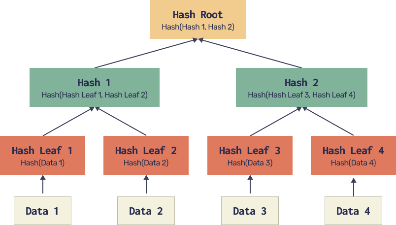
A file is split into many parts (Data 1,…,Data 4 on our diagram). We hash each part to get a digest, then we hash pairs of digests, then we hash pairs of hashes, etc. until we get one single hash. This hash root is published on the internet as the file identifier. Now, when you download a part of the file it comes with a number of hashes that allow verification of this part’s consistency with the published hash root.
For instance, when we download Data 3, it comes with Hash Leaf 4 (but not Data 4) and Hash 1. Once Data 3 is downloaded, we can hash it, then use Hash Leaf 4 to compute Hash 2 and then use Hash 1 together with the computed Hash 2 to get the Hash Root. If it matches the published one, chances are high that our Data 3 piece is genuine. In fact the properties of a hash function, precisely the implausibility of finding another input that produces the same hash, ensure the impossibility of forging a selected part of the file, while keeping the same hash root.
Finally, back to polynomials. The setting is in fact quite similar to file torrents. We have polynomial values ( = Data fragments) that we want to learn while being sure they all come from the same polynomial ( = entire file). The subtle difference is that, unlike the file, we don’t expect to learn the entire polynomial eventually, but the construction provides guarantees for each individual fragment regardless of the ultimate goal. So, what we might do is organize something similar to a Merkle tree for values of a polynomial with the hash root corresponding to the entire polynomial.
While this idea has some technical caveats, it is generally feasible. Such a construction is called a commitment scheme for a polynomial. A polynomial is linked to a digest in a way that allows to check any communicated value to come from this exact polynomial. While real constructions of commitment schemes are more complicated than simple Merkle trees, or may even be based on completely different ideas not involving hashes, the general principle remains the same. Every polynomial has a digest - a commitment - that prevents the prover from faking information about the values of this polynomial at specific points.
Programming in a spreadsheet
We now finally get to the part where we deal with the program we want to delegate. In order to transform it into a proof (i.e. a mathematical puzzle with a solution) we will have to encode the program in a rather unconventional way. When we say “program” we don’t mean something with fancy 3D graphics and multichannel sound but rather a set of instructions that transforms some input into some output. A program should be deterministic, i.e. if we fix an input we always get the same output, however many times we run it. That’s pretty much what one would expect from a decent program entrusted with a serious task.
The promised unconventional transformation of the program consists in encoding the program by means of polynomials. The idea behind it is to use all the polynomial magic we devised above. Yet, transforming an arbitrary set of instructions into polynomials is far from anything people do on a daily basis. To keep things simple we’ll stick to outlining the general idea and providing some simple examples. Precisely our goal is to represent a computer program as a table (think of a spreadsheet) and a number of equations for the table cells. The equations are meant to ensure the values of input cells define uniquely the output cells. All this (table + equations) is called a circuit for a rather obscure reason we shall not address here.
This next part will probably be rather technical, so once you’re bored, you can probably… take a break and then try once again? If that doesn’t help, you can go with a leap of faith and just assume that any program relating an input to an output can indeed be encoded as a set of polynomials that all have a predefined list of guaranteed roots. Once you’re ready to believe that, you can simply jump to the next section. Should you feel ready for seemingly pointless manipulations of algebraic expressions, please carry on.
If you got so far into the text, you’re probably aware that computers count in bytes and each byte is made up of 8 bits. If that’s a novel concept for you, make sure to google it before you read on. For an example circuit we’ll design one that computes the parity of a number using decomposition of a byte into bits.
The input for this program is a number that fits into a byte, and the output is 0 or 1, depending on the input’s parity. This output is exactly the input’s lowest bit. In order to achieve that we’ll use some intermediary values. Precisely, we’ll put the number’s bit decomposition into the cells of a table. We’ll put the number itself into cell A1, fill in its bits into the cells B1…E2 and put the result into cell A2. For instance, if the input number is 185, the table is as follows.
Now, we’ll write equations that relate the cells of this table. A1 is related to B1...E2 via:
A1 = B1 + 2C1 + 4D1 + 8E1 + 16B2 + 32C2 + 64D2 + 128*E2
The resulting cell A2 is simply a copy of B1:
A2 = B1
Finally, the cells B1…E2 may only contain 0’s and 1’s. This is ensured by the following equations.
All these equations together are called constraints and they are exactly what defines the circuit. They are the algebraic representation of the operation “compute the parity of a number”. A non-trivial, non-exciting yet necessary exercise is to check that these equations allow no other solution besides the one that we expect. If they happen to allow (which is not our case fortunately) the circuit is called under-constrained and it is something that might allow a malevolent prover to prove a false statement: in our case - claim false parity for the input number.
How do all these equations actually become a mathematical puzzle, a proof that we indeed filled the table in accord with all the constraints? Well, we’ll need more polynomials. We’ll start by writing the values in each table column as a polynomial. The variable will be the row number $r$. For column A we’ll have polynomial $A$:
$$A = (2-r)\cdot A1 + (r-1)\cdot A2$$
When $r = 1$ we get
$$A = (2-1)\cdot A1 + (1-1)\cdot A2 = A1$$
and when $r = 2$ we get
$$A = (2-2)\cdot A1 + (2-1)\cdot A2 = A2.$$
Obviously we can thus construct a polynomial for every column. Less obvious, but still true, it is still feasible if we have more than two rows or if we prefer some other numbering for the rows. The latter is especially relevant because in proving real circuits we prefer to have rows numbered by some specially chosen elements.
Now we can deal with polynomials in the variable $r$, one for each table column: $A, B, C, D, E$. Using those, we can simplify each pair of equations we have for columns B,..,E into something more concise. In fact the “bit” constraints for cells in B1,..,E2 translate into equations:
$$B(B-1) = 0,\quad C(C-1) = 0,\quad D(D-1)=0,\quad E(E-1) = 0$$
with left-hand sides being polynomials in the variable $r$. These equations should hold for $r = 1$ and $r = 2$ in our case, and for every row label in the more general case. Transforming the two remaining constraints into expressions with column polynomials requires a little more tweaking. Because these constraints relate cells in different rows, the column polynomials by themselves do not suffice. The usual trick is to construct another column polynomial for a “shifted” column.
Just like we would construct a polynomial $C$ for a column with values C1,C2,C3,….C9C10 (for instance), we can construct a shifted polynomial $\vec{C}$ for a column with values C10,C1,C2,C3,…,C9. In our specific case with just two rows, the polynomial $\vec{B}$ will be the simple yet possibly misleading expression: $(2-r)\cdot B2 + (r-1)\cdot B1$. Using this $\vec{B}$ polynomial we can construct the following expression to encompass the constraint A2 = B1:
$$A - \vec{B} = 0.$$
When we expand it, we actually get:
$$(2-r)\cdot A1 + (r-1) \cdot A2 - (2-r)\cdot B2 - (r-1)\cdot B1 = 0.$$
Now, substituting $r = 1$ and $r = 2$ into that produces
$$A1 - B2 = 0\text{ and } A2 - B1 = 0,$$
which is a little more than what we bargained for. Excluding the extraneous constraint $A1-B2 = 0$ can be achieved by multiplying the initial relation by $(r-1)$:
$$(r-1)\cdot (A - \vec{B}) = 0$$
translates exactly into
$$(r-1)\cdot(2-r)\cdot(A1-B2) + (r-1)\cdot(r-1)(A2 - B1) = 0,$$
which gives us the always-satisfied $0 = 0$ for $r = 1$ and the sought-after $A2-B1 = 0$ for $r = 2$. Finally, the longest constraint which defines the cell A1, can be written as follows:
$$(2-r)\cdot (A - B - 2C - 4D -8E - 16\vec{B} - 32\vec{C} - 64\vec{D} - 128\vec{E}) = 0.$$
A not-so-lazy reader can check that this indeed translates into the initial A1 constraint for $r = 1$ and becomes $0 = 0$ when $r = 2$.
We finally arrive to the point where we have listed all the basic tricks to encode our computations as polynomials. Believe it or not, everything your computer can do may eventually be written as a table with constraints. (This table might be too big to fit in the memory of any existing computer, but who cares!) The table cells are constrained by polynomial relations. These should hold for every row label $r$ only if the table is filled with values that represent a valid computation for our chosen relation between the input and output.
At this point, we’ve turned computation into math: a program is no longer something you run, but something you check through constraints and polynomials.
We’ll get to that in Part II of this article, where we’ll show how this entire structure can be verified with a single randomized check. See you next week!